Leetcode 1368. Minimum Cost to Make at Least One Valid Path in a Grid

 1368. Minimum Cost to Make at Least One Valid Path in a Grid

Hard, Arrays,

Dynamic Programming

Given an m x n grid. Each cell of the grid has a sign pointing to the next cell you should visit if you are currently in this cell. The sign of grid[i][j] can be:

• 1 which means go to the cell to the right. (i.e go from grid[i][j] to grid[i][j + 1])
• 2 which means go to the cell to the left. (i.e go from grid[i][j] to grid[i][j - 1])
• 3 which means go to the lower cell. (i.e go from grid[i][j] to grid[i + 1][j])
• 4 which means go to the upper cell. (i.e go from grid[i][j] to grid[i - 1][j])

Notice that there could be some signs on the cells of the grid that point outside the grid.

You will initially start at the upper left cell (0, 0). A valid path in the grid is a path that starts from the upper left cell (0, 0) and ends at the bottom-right cell (m - 1, n - 1) following the signs on the grid. The valid path does not have to be the shortest.

You can modify the sign on a cell with cost = 1. You can modify the sign on a cell one time only.

Return the minimum cost to make the grid have at least one valid path.

 

Example 1:

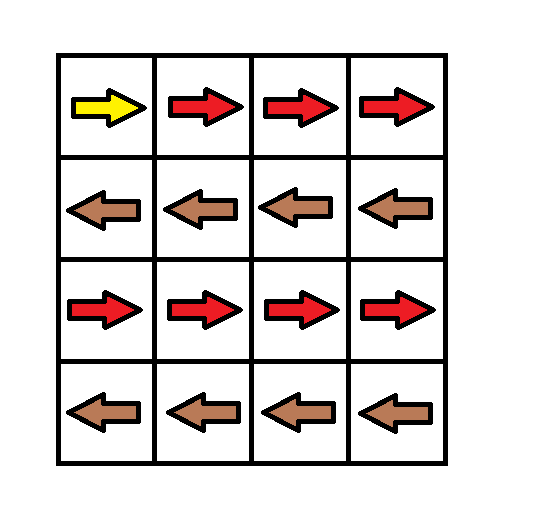
Input: grid = [[1,1,1,1],[2,2,2,2],[1,1,1,1],[2,2,2,2]]
Output: 3
Explanation: You will start at point (0, 0).
The path to (3, 3) is as follows. (0, 0) --> (0, 1) --> (0, 2) --> (0, 3) change the arrow to down with cost = 1 --> (1, 3) --> (1, 2) --> (1, 1) --> (1, 0) change the arrow to down with cost = 1 --> (2, 0) --> (2, 1) --> (2, 2) --> (2, 3) change the arrow to down with cost = 1 --> (3, 3)
The total cost = 3.

Example 2:

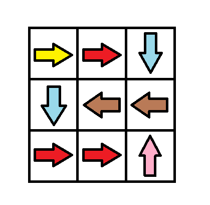
Input: grid = [[1,1,3],[3,2,2],[1,1,4]]
Output: 0
Explanation: You can follow the path from (0, 0) to (2, 2).

Example 3:

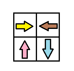
Input: grid = [[1,2],[4,3]]
Output: 1

 

Constraints:

• m == grid.length
• n == grid[i].length
• 1 <= m, n <= 100
• 1 <= grid[i][j] <= 4

Problem Statement:

You are given an $m \times n$ grid, where each cell contains a sign directing the next move. The signs are:

1. 1: Move right.
2. 2: Move left.
3. 3: Move down.
4. 4: Move up.

You start at the top-left cell (0, 0) and aim to reach the bottom-right cell $(m-1, n-1)$. You can change the sign on any cell at a cost of 1. The goal is to determine the minimum cost to make at least one valid path from $(0, 0)$ to $(m-1, n-1)$.

---

Approach Explanation:

This problem can be tackled using a modified version of Dijkstra's algorithm. The key idea is to minimize the cost of traversing the grid to reach the destination. Here's the step-by-step approach:

---

1. Understanding Movement Costs:

• Moving in the direction indicated by the current cell's sign costs 0.
• Changing the direction to any other valid move costs 1.

---

2. Data Structures:

• Use a priority queue to always process the cell with the smallest cost first.
• Maintain a cost array to track the minimum cost required to reach each cell.

---

3. Algorithm:

1. Initialization:

   • Start with the top-left cell $(0, 0)$ with cost 0.
   • Push this cell into the priority queue.

2. Process Cells:

   • For each cell, explore all possible directions:
     • If moving in the indicated direction:
       • Add it to the queue with no additional cost.
     • If moving in another direction:
       • Add it to the queue with cost + 1.

3. Stop Early:

   • If you reach the bottom-right cell $(m-1, n-1)$, return the cost.

4. Terminate:

   • The priority queue ensures cells with the smallest cost are processed first, guaranteeing the minimum cost to reach the destination.

---

Solution in C#:

using System;
using System.Collections.Generic;

public class Solution {
    public int MinCost(int[][] grid) {
        int m = grid.Length, n = grid[0].Length;
        int[][] directions = new int[][] {
            new int[] {0, 1},  // right
            new int[] {0, -1}, // left
            new int[] {1, 0},  // down
            new int[] {-1, 0}  // up
        };
        
        int[,] cost = new int[m, n];
        for (int i = 0; i < m; i++)
            for (int j = 0; j < n; j++)
                cost[i, j] = int.MaxValue;

        var pq = new PriorityQueue<(int row, int col, int cost), int>();
        pq.Enqueue((0, 0, 0), 0);
        cost[0, 0] = 0;

        while (pq.Count > 0) {
            var (x, y, c) = pq.Dequeue();
            
            if (x == m - 1 && y == n - 1)
                return c;

            if (c > cost[x, y])
                continue;

            for (int k = 0; k < 4; k++) {
                int nx = x + directions[k][0];
                int ny = y + directions[k][1];
                int newCost = c + (k + 1 == grid[x][y] ? 0 : 1);

                if (nx >= 0 && nx < m && ny >= 0 && ny < n && newCost < cost[nx, ny]) {
                    cost[nx, ny] = newCost;
                    pq.Enqueue((nx, ny, newCost), newCost);
                }
            }
        }

        return -1; // Should not reach here
    }
}

---

Example Walkthrough:

Input:

grid = [[1,1,1,1],
        [2,2,2,2],
        [1,1,1,1],
        [2,2,2,2]]

Execution:

1. Start at (0, 0) with cost = 0.
2. Move along the indicated path:
   • $(0, 0) → (0, 1) → (0, 2) → (0, 3)$.
3. Change the arrow at $(0, 3)$ to go down $(cost = 1)$.
4. Continue:
   • $(1, 3) → (2, 3) → (3, 3)$.
5. Change arrows at $(1, 0)$ and $(2, 0)$, costing an additional 2.

Output:

Cost = 3

---

Complexity Analysis:

1. Time Complexity:
   • $O(m \cdot n \cdot \log(m \cdot n))$: The priority queue processes each cell once, with logarithmic operations for insertion and deletion.
2. Space Complexity:
   • $O(m \cdot n)$: For the cost array and the priority queue.

---

 While the priority queue-based solution (modified Dijkstra's algorithm) is an optimal approach for this problem, I'll also include other potential approaches. Each method has its own advantages and trade-offs, and their inclusion provides a more comprehensive understanding of the problem-solving strategies.

---

Alternate Approaches:

1. Breadth-First Search (BFS) with a Deque:

• Idea: Instead of using a priority queue, use a double-ended queue (deque) to implement a 0-1 BFS.
• How it works:
  • Push cells with a cost of 0 to the front of the deque.
  • Push cells with a cost of 1 to the back of the deque.
• Advantages: This avoids the overhead of maintaining a heap (priority queue), making it faster in practice for grid-based problems.
• Complexity:
  • Time: $O(m \cdot n)$ because each cell is processed at most once.
  • Space: $O(m \cdot n)$.

Implementation:

using System;
using System.Collections.Generic;

public class Solution {
    public int MinCost(int[][] grid) {
        int m = grid.Length, n = grid[0].Length;
        int[][] directions = new int[][] {
            new int[] {0, 1},  // right
            new int[] {0, -1}, // left
            new int[] {1, 0},  // down
            new int[] {-1, 0}  // up
        };

        int[,] cost = new int[m, n];
        for (int i = 0; i < m; i++)
            for (int j = 0; j < n; j++)
                cost[i, j] = int.MaxValue;

        var deque = new LinkedList<(int x, int y, int c)>();
        deque.AddFirst((0, 0, 0));
        cost[0, 0] = 0;

        while (deque.Count > 0) {
            var (x, y, c) = deque.First.Value;
            deque.RemoveFirst();

            if (c > cost[x, y]) continue;

            for (int k = 0; k < 4; k++) {
                int nx = x + directions[k][0];
                int ny = y + directions[k][1];
                int newCost = c + (k + 1 == grid[x][y] ? 0 : 1);

                if (nx >= 0 && nx < m && ny >= 0 && ny < n && newCost < cost[nx, ny]) {
                    cost[nx, ny] = newCost;
                    if (k + 1 == grid[x][y])
                        deque.AddFirst((nx, ny, newCost));
                    else
                        deque.AddLast((nx, ny, newCost));
                }
            }
        }

        return cost[m - 1, n - 1];
    }
}

---

2. Dynamic Programming (DP):

• Idea: Use a dynamic programming table dp[i][j] where each cell represents the minimum cost to reach that cell.
• How it works:
  • Start from the top-left cell $(0, 0)$.
  • Iteratively update the minimum cost for each cell by checking all possible directions.
  • Use multiple iterations until no further updates can be made.
• Advantages: Intuitive to implement and easy to reason about.
• Disadvantages: Less efficient for large grids, as it may require multiple iterations to propagate the cost values.
• Complexity:
  • Time: $O(k \cdot m \cdot n)$, where $k$ is the number of iterations (can be up to $m \cdot n$ in the worst case).
  • Space: $O(m \cdot n)$.

Implementation:

public class Solution {
    public int MinCost(int[][] grid) {
        int m = grid.Length, n = grid[0].Length;
        int[][] directions = new int[][] {
            new int[] {0, 1},  // right
            new int[] {0, -1}, // left
            new int[] {1, 0},  // down
            new int[] {-1, 0}  // up
        };

        int[,] dp = new int[m, n];
        for (int i = 0; i < m; i++)
            for (int j = 0; j < n; j++)
                dp[i, j] = int.MaxValue;

        dp[0, 0] = 0;
        bool updated = true;

        while (updated) {
            updated = false;
            for (int i = 0; i < m; i++) {
                for (int j = 0; j < n; j++) {
                    for (int k = 0; k < 4; k++) {
                        int ni = i + directions[k][0];
                        int nj = j + directions[k][1];
                        if (ni >= 0 && ni < m && nj >= 0 && nj < n) {
                            int newCost = dp[i, j] + (grid[i][j] == k + 1 ? 0 : 1);
                            if (newCost < dp[ni, nj]) {
                                dp[ni, nj] = newCost;
                                updated = true;
                            }
                        }
                    }
                }
            }
        }

        return dp[m - 1, n - 1];
    }
}




---

Comparison of Approaches:

Approach	Time Complexity	Space Complexity	Pros	Cons
Priority Queue (Dijkstra)	$O(m \cdot n \cdot \log(m \cdot n))$	$O(m \cdot n)$	Optimal for weighted shortest path problems.	Overhead of maintaining a heap.
BFS with Deque (0-1 BFS)	$O(m \cdot n)$	$O(m \cdot n)$	Faster for grid problems with unit costs.	Harder to understand than Dijkstra.
Dynamic Programming (DP)	$O(k \cdot m \cdot n)$	$O(m \cdot n)$	Intuitive and easy to implement.	Can be slower for large grids.

---

Including multiple approaches not only provides flexibility in implementation but also helps understand different paradigms for solving grid-based pathfinding problems.